Simulator Characteristics

IPARS supports three dimensional transient flow of multiple phases containing multiple components plus immobile phases (rock) and adsorbed components. The nonlinear partial differential equations describing flow are solved by cell-centered finite-difference methods in the current version of the simulator but the use of finite-element methods in future versions is not excluded.

Phase densities and viscosities may be arbitrary functions of pressure and composition or may be represented by simpler functions (e.g. constant compressibility). Actual treatment of phase properties depends on the physical model.

Porosity (at standard conditions) and permeability may vary with location in an arbitrary manner. Some physical models treat porosity as a constant and others make it a function of pressure. Permeability is currently a constant diagonal tensor but provision is made for using a full tensor.

Relative permeability, and capillary pressure are functions of saturations and rock type. Rock type is a function of location. Several models for three-phase relative permeability are built into the simulator and other models can be added as needed. Any dependence of relative permeability and capillary pressure on composition and pressure is left to the individual physical models.

IPARS provides a general x-y function capability that is widely used in the physical models to represent various properties; the options in this capability include:

1. Piecewise constant
2. Piecewise linear
3. Quadratic spline with optional poles
4. Cubic spline with optional poles
5. User define functions (FORTRAN code in the input data)

Yes, the simulator includes a built-in compiler which can be convenient when one wants to use an analytic function to represent, say, the dependence of relative permeability on water saturation.

The reservoir consists of one or more fault blocks. Each fault block has an independent user-defined coordinate system and gravity vector. Flow between fault blocks can occur wherever fault blocks share a common face. The primary grid imposed on each fault block is a logical cube but may be geometrically irregular. Grid elements may be keyed out to represent irregular shapes and impermeable strata. The grid may also be distorted to represent curved formations; the small-angle approximation is used for this purpose.

The simulator currently supports three-dimensional rectangular Cartesian grids in most cases. There are capabilities to execute two-phase flow simulations on unstructured grids using discontinuous Galerkin methods. A simple grid for a single fault block is illustrated in Fig. 1. Two columns of grid elements have been keyed out in the figure to demonstrate a method that can be used to represent irregularly shaped reservoirs or aquifers. Multiple fault with independent grids may also be specified. Flow can occur between fault blocks that share a common surface. This surface does not have to be parallel to a coordinate plain but may instead be formed by keying out elements in the two blocks. The name "fault block" is somewhat misleading; there are other uses for the IPARS geometric capability. One may, for example, key out a column of elements containing a well and replace the column with a "fault block" having a finer grid. To take the process one step farther, one might also specify the black-oil for the inner fault block and the two-phase model for the outer fault block.

On multiprocessor machines, the grid system is distributed among the processors such that each processor is assigned a subset of the total grid system. The subgrid assigned to a processor is surrounded by a "communication" layer of grid elements that belong to other processors. The framework provides a routine that updates data in the communication layer.

IPARS supports an arbitrary number of wells each with one or more completion intervals. A well may penetrate more than one fault block but a completion interval must occur in a single fault block. On parallel machines, well grid elements may be assigned to more than one processor. For each well element, the framework provides estimates of the permeability normal to the wellbore, the geometric constant in the productivity index, and the length of the open interval. Other well calculations are left to the individual physical models.

Portability of the simulator is emphasized. FORTRAN77 and classical C code are used. Manufacturer specific language enhancements are prohibited. Commercial libraries are also prohibited except in the graphics area.

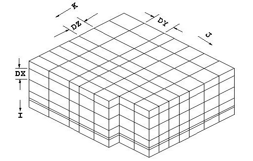
A Simple IPARS Grid

A restart capability is included in IPARS. The restart file(s) are independent of the number of processors and may be written in either binary or ASCII format. An ASCII file is much larger than the same file written in binary but can be moved between machines and operating systems.

Free-form keyword input is used by the simulator. The input file can be prepared with any editor capable of producing an ASCII file. Much of this manual is devoted to defining keyword variables.

Multiple levels of output are provided in the simulator. These range from selective memory dumps for debugging to minimal output for automatic history matching. Every output statement in the simulator is assigned an output level. The simulator will not, repeat not, dump all results between time steps so that the user can choose any output he pleases after the simulation.

Internally the simulator uses a single set of units for each physical model. Externally, the user may choose any physically correct units he pleases; if he wants to specify production rates in units of cubic furlongs per fortnight, the simulator will determine and apply the appropriate conversion factor. The simulator does provide a default set of external units for each physical model.